Abstract
An alternate approach is presented where graphing discharge can be accomplished without a time axis. This technique allows data properties such as Q, dQ/dt, and d2Q/dt2, and trends of increasing, decreasing or no change flow to be readily seen and understood on a single graph. Flow pulse reference lines can easily be added and interpreted. The methodology is based on the time-series serial correlation lag-1 graph and uses the normally unwanted (but still valuable) autocorrelation present within the streamflow data. Examples and applications are included.
Key words: Lag-1 hydrograph, autocorrelation, 1st, 2nd order derivative, hydrograph analysis
Introduction
Hydrographs are an essential tool for hydrologists or other water resources professionals. The USGS defines a hydrograph as “a graph showing stage, flow, velocity, or other property of water with respect to time.” (Langbein and Iseri, 1960). Note there is no rigid requirement that a time axis be used when plotting time-base data, though this is the most common method. Another approach is demonstrated in this paper.
Lag-1 Hydrograph Method
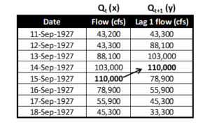
Data preparation and plotting are identical to an autocorrelation lag 1 plot, where 1 indicates a 1-day time shift. Table 1 shows how the time-series discharges are shifted. For this paper, the unshifted discharge is labeled Qt (the x coordinate) and the shifted discharge Qt+1 (the y coordinate). It is critical that the temporal sequence is maintained for the data. Thinking of the x values as “flow for today” and the y values as “flow for tomorrow” helps to visualize the order of the data.
Table 1. Data shift example (USGS site Colorado River at Lees Ferry, AZ)
To calculate discharge change, a ratio between the coordinates is used. This ratio can be used as a reference on the plot. For these equations below, the (x,y) coordinate is (Qt, Qt+1). In all cases there is a 1-day time step so that the change in time (Dt) is 1.
Equation 1a y = mx
Equation 1b Qt+1 = m Qt
where m = change ratio
Equation 2 m = y/x = (Qt+1) / (Qt)
where m > 1, discharge is increasing
m = 1, no change to discharge
m < 1, discharge is decreasing
Equation 3a y – x = Qt+1 – Qt = DQ/day
Equation 3b (m – 1) Qt = Qt+1 – Qt = DQ/day
A traditional line hydrograph for the data in Table 1 is shown in Figure 1.
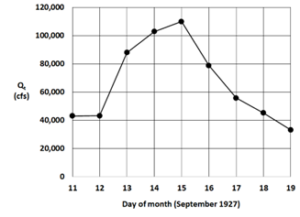
Figure 1. Line hydrograph for the Colorado River at Lees Ferry, AZ
The hydrograph represents runoff from a Pacific hurricane remnant that crossed into the southwestern United States (Weaver, 1968). The multiday event provides a useful example to display and discuss properties of the Lag-1 hydrograph.
A key item with this approach is that time is employed as a data attribute rather than as a coordinate. The lag-1 hydrograph (Figure 2) allows for additional information such as regions of increasing, decreasing or no change in discharge. An interesting feature of this plot is that the first and second order derivatives of the discharge are displayed.
Consider the following data representations on a Lag-1 hydrograph:
1. The x coordinate of a data point represents the daily discharge (Qt)
2. Each data point represents DQ/day or dQ/dt (1st order derivative)
3. Lines connecting points represent D(DQ/day) or d2Q/dt2 (2nd order derivative)
The details listed above are comparable to distance (item 1), velocity (item 2), and acceleration (item 3) from the physics of motion. Regions are highlighted below.
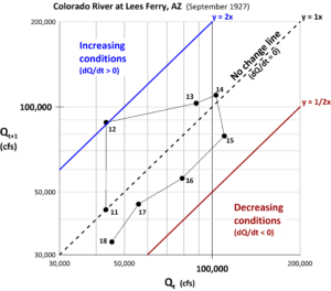
Figure 2. Lag-1 hydrograph example (day number associated with Qt).
Results
Figures 1 and 2 use the same data but display very different graphics.
Below are detailed comparisons of the two plots:
Days 11 to 12 – The line hydrograph shows little change between these two days, while the lag-1 hydrograph shows a single point very close to the y = 1x ratio change line.
Days 12 to 13 and 13 to 14 – The line hydrograph shows the rising limb of the event. The lag-1 hydrograph shows days 11, 12, 13, and 14 are all above the 1x line, indicating rising flow conditions. But because the distance of the points decreases from the 1x line, this shows the increases are occurring, but at a decreasing rate. Day 14 shows the peak for Qt+1, while Day 15 shows the peak for Qt. Both represent the discharge on 15 Sept 1927.
Days 15, 16, 17 and 18 – the line hydrograph shows decreasing flows. The lag-1 hydrograph also shows the decreasing flow conditions as all points are below the 1x line.
Additionally, the rate of change for the decrease is consistent. A power curve fitted to these points yields a recession equation for the general form aQb where Qt+1 = 1.8124 Qt 0.9198. This is consistent with the extraction method of baseflow recession segments based on a second-order derivative (Yang, et al., 2020).
Discussion & Conclusion
This paper is a brief overview of a new technique that does not appear elsewhere in the published literature. Here are three ways this technical approach can be used in water resources projects. First – use this method for model calibration by having the x axis be the observed data and the y axis be the modeled data. The resulting plot would be an “error hydrograph” showing time and discharge differences. Next – scale up the data used from one runoff event to a multi-year discharge record with the x axis as Qt and the y axis as Qt+1. The resulting plot becomes an autocorrelation lag 1 plot but now with the Q, dq/dt and d2Q/dt2 regions. Additionally, the autocorrelation r(k), a metric of persistence and randomness, can be calculated. Finally – let an upstream gaging station be the x axis and a downstream station, lagged by the routing time, be the y axis. The resulting plot will show the contribution of the local, ungaged area between the two stations.
A more in-depth treatment of this novel approach is available as a webinar (June 16, 2022) sponsored by the American Institute of Hydrology (AIH webinar, 2022).
Remarks
The author thanks AIH for the opportunity to share this self-funded research.
References
AIH webinar. 2022. A Novel Approach to Quantify Streamflow Properties, https://www.aihydrology.org/aih-webinar-a-novel-approach-to-quantify-streamflow-properties/
Langbein, W. B., and Iseri, Kathleen T., 1960. General Introduction and hydrologic definitions: U.S. Geol. Survey Water-Supply Paper 1541-A, 29 p.
Weaver, R. 1968. Meteorology of Major Storms in Western Colorado and Eastern Utah. Technical Memorandum WBTM HYDRO-7. U.S. Dept. of Commerce, Environmental Science Services Administration, Weather Bureau.
Yang, W., C. Xiao, and X. Liang. 2020. Extraction Method of Baseflow Recession Segments Based on Second-Order Derivative of Streamflow and Comparison with Four Conventional Methods. Water. 12. 10.3390/w12071953.
About the Author
Dr. Koehler is the CEO of Visual Data Analytics and a certified professional hydrologist with over 40-years’ experience.
Previously he was the National Hydrologic and Geospatial Sciences Training Coordinator for NOAA’s National Weather Service and is a retired NOAA Corps lieutenant commander. Assignments included navigation and operations officer for two NOAA oceanographic research ships, the Colorado Basin River Forecast Center and the Northwest River Forecast Center where he oversaw the implementation of an operational dynamic wave model for Lower Columbia River stage forecasts. Other positions include Director of Water Resources for an Arizona consulting company and the water resources hydrologist for Cochise County, Arizona.
He is also a member of the science department faculty at Front Range Community College and is instructor for astronomy, geology, geography, GIS and geodesy courses. He is also an FAA certified professional drone operator.
He has a PhD, MS and BS in Watershed Management from the University of Arizona and an additional MS in Hydrographic Sciences from the US Naval Postgraduate School. The focus of his research are alternate methods of analyzing environmental time-series data along with associated data visualizations.


 This is an overdue update to our AIH members and community about what your AIH leadership team has been up to this year. I am thrilled to announce completion of critical and timely updates to the governing documents for our organization – our AIH Articles of Incorporation (formerly, Constitution) and AIH Bylaws. We initiated the review and update process in 2016. Over the past six years, past and current AIH leadership team members devoted many, many hours to completing a comprehensive review and developing suggested revisions to these documents. This review and update provided a great opportunity to reflect on how we have operated and how we will function in the future. In the spirit of these changes, Leonardo Da Vinci once remarked (translated to English): “When you put your hand in a flowing stream, you touch the last that has gone before and the first of what is still to come.” It is extremely gratifying to see the results of our review/update process in our new governing documents, and I look forward to the next steps.


 About The Speaker: Andrew Cohen is a hydrogeologist located in New Jersey, USA. He received a Ph.D. from the University of California at Berkeley. His focus is hydrogeologic investigations, contaminant fate and transport, conceptual site models, and groundwater education. Prior to his current roles in the environmental consulting industry and Adjunct Professor of Contaminant Hydrogeology at the New Jersey Institute of Technology, he was a Research Associate at Lawrence Berkeley National Laboratory, where he focused on hydrogeologic characterization and modeling of groundwater in fractured and faulted bedrock. He is now focused on the development of a free, online library of groundwater educational videos called the GroundwaterU Video Library, which he founded in January of this year.