Skip to content

A Climate Condition Analysis Using Palmer Hydrologic Drought Index (PHDI) values

A Climate Condition Analysis Using Palmer Hydrologic Drought Index (PHDI) values

Richard Koehler, PhD, PH, CEO, Visual Data Analytics, LLC  visual.data.analytics@outlook.com


Abstract

Drought and climate change are important factors to include in any hydrologic analysis. Current weather-related events in California, such as the extended drought and recent multiple atmospheric rivers, demonstrate how quickly hydrologic conditions can change. A lag(1) autocorrelation analysis of California Climate Division 2 (Sacramento Drainage) using monthly Palmer Hydrologic Drought Index (PHDI) values was conducted to find data ranges, persistence of conditions, along with seasonal and historical drought patterns. Results show distinct conditions within the hydrologic-climatic system which include periods of (a) persistent drought, (b) persistent wet, (c) transition from drought to wet, and (d) transition from wet to drought. Month-to month PHDI changes are quantified using a summation infographic based on the autocorrelation scatterplot.

Key words: PHDI, drought, lag(1) autocorrelation


Background

California is divided into seven climate divisions, each with various types of climate indices (Figure 1). For this study, Climate Division 2, Sacramento River drainage (NOAA, 2023a) is used as it contains the Lake Shasta reservoir, an important component of California’s water resources system.

This study examined PHDI information produced by NOAA’s National Centers for Environmental Information (NCEI). The NOAA website for drought data states that the PHDI “measures hydrological impacts of drought (e.g., reservoir levels, groundwater levels, etc.) which take longer to develop and longer to recover from. This long-term drought index was developed to quantify these hydrological effects, and it responds more slowly to changing conditions than the Palmer Drought Severity Index” (NOAA, 2023b). Table 1 describes the different PHDI levels (Hayes, 2007) and Figure 2 shows the 1895 to 2023 timeline plot of this monthly data  (NOAA, 2023c).

Some of the most severe drought values have occurred in recent years, with June 2021 through September 2021 all exhibiting PHDI values in the extreme drought range (-5 or more negative).

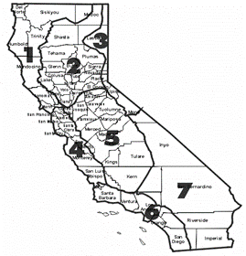
Figure 1: California Climate Divisions,

Climate Division 2, Sacramento River drainage (source: NOAA).

Table 1: PHDI level descriptions (Hayes, 2007).

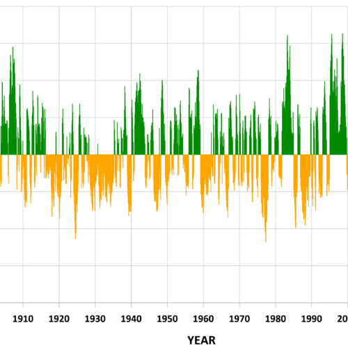
Figure 2: California Climate Division 2,  monthly PHDI values, 1895 to 2023 (source: NOAA).

A histogram (Figure 3) shows the number of months for each PDHI value. There is a distinct bimodal distribution, with a total of 804 months of drought conditions (negative PHDI) and 661 months of wet conditions (positive PHDI). The 0 condition (near normal) represents only 15 months, indicating that this rarely occurred.

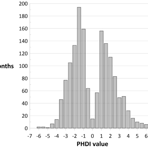
Figure 3: California Climate Division 2,  PHDI histogram – months per PHDI condition.

Analysis technique

A lag (1) temporal autocorrelation scatterplot was used to examine the PHDI data. Table 2 shows the one-month data shift used to create an x-y system with PHDI at time “t” for the x coordinate,  and PHDI at time “t+1” for the y coordinate.

Table 2: PHDI one-month data shift example.

Results

Extremes can be represented by large positive and large negative monthly PHDI changes, shown in the following tables (Tables 3 and 4).

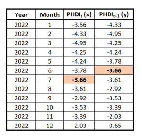
Table 3: Ranked largest positive monthly PHDI changes, California Climate Division 2.

Table 4: Ranked largest negative monthly PHDI changes, California Climate Division 2.

However, this simple approach provides an incomplete view of how the hydrologic-climatic system operates. A more expansive approach is to graph all monthly changes with a lag(1) autocorrelation scatterplot (Figure 4), where each point represents the monthly PHDI change.

Any point on the dashed diagonal line (y = 1x) indicates no PHDI change from month-to-month. Any point above the diagonal line signifies positive PHDI changes, while any point below the diagonal line signifies negative PHDI changes. Additionally, the overlay shows groups of points that represent four components of the hydrologic-climatic system, (a) persistent drought, (b) persistent wet, (c) transition from drought to wet, and (d) transition from wet to drought. The Table 1 description for “near normal” (-0.49 to +0.49) rarely happened, as the hydrologic system constantly oscillates between persistent drought and persistent wet conditions.

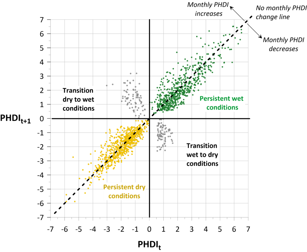
Figure 4: PHDI lag(1) autocorrelation scatterplot with four conditions.

As each point can be identified by month, a breakout of seasonal scatterplots is possible as shown in Figure 5.

Spring and summer have fewer transitions. These two seasons also have less overall scatter, indicating more persistent wet and dry conditions. Interestingly, summer has both the driest and some of the wettest PHDI values. Winter and fall show more randomness, as data points are more scattered. These two seasons also have more transition points. Atmospheric rivers typically occur during winter (NASA 2023) but, with transition points seen in all four seasons, other mechanisms are likely in play.

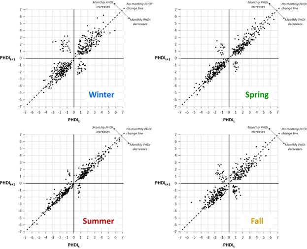
Figure 5: Seasonal autocorrelation scatterplots, (a) winter, (b) spring, (c) summer, (d) fall.

PHDI values were rounded to the nearest 0.5 to provide a consistent way to compare all month-to-month pairings, allowing for a summation of all changes for the period of record: 1895 to 2023 (Figure 6).

The PHDI value of -3 shows the single greatest range of change, -4 to +2.5 (Figure 6a). This display helps identify the most and least common changes that have taken place. The most common value is the monthly PHDI value of -1.5 followed by -1.5, which occurred 81 times (Figure 6b). Summation values of 1 indicate unusual conditions as these specific monthly changes occurred only once in the 128-year record.

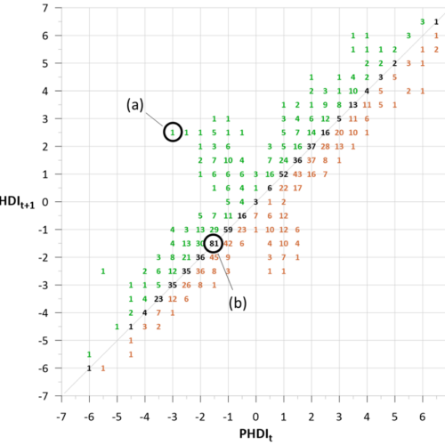
Figure 6: Historical summation of all PHDI monthly changes for California Climate Division 2:

(a) single largest change, (b) most common month-to-month occurrence.

Coordinates for count values are based on categorized PHDI values.

Conclusions

The lag(1) autocorrelation scatterplot provides a basis for additional information about climatic datasets not possible with other methods. The identification of four distinct components of the hydrologic-climatic system provides new opportunities for planning and management activities by water resource organizations. The success of this approach suggests that more research should be directed to looking into mechanisms that enable large PHDI changes.

For more information about the Lag-1 autocorrelation, please read Dr. Koehler’s previous article, titled “The Lag-12 Hydrograph – Alternate Way to Plot Streamflow Time-Series Data”, AIH Bulletin, Fall 2022.


References

Hayes, M. J., 2007. Drought Indices.

https://wwa.colorado.edu/sites/default/files/2021-09/IWCS_2007_July_feature.pdf

NOAA, 2023a. Location of US Climate Divisions. https://psl.noaa.gov/data/usclimdivs/data/map.html

NOAA, 2023b. Historical Palmer Drought Indices.

https://www.ncei.noaa.gov/access/monitoring/historical-palmers/overview

NOAA, 2023c. Climate at a Glance Divisional Time Series. https://www.ncei.noaa.gov/access/monitoring/climate-at-a-glance/divisional/time-series/0402/phdi/all/3/1895-2023?base_prd=true&begbaseyear=1901&endbaseyear=2000

NASA, 2023. Atmospheric Rivers

https://ghrc.nsstc.nasa.gov/home/micro-articles/atmospheric-rivers


About the author

Dr. Koehler is the CEO of Visual Data Analytics and a certified professional hydrologist with over 40-years’ experience.

Previously he was the National Hydrologic and Geospatial Sciences Training Coordinator for NOAA’s National Weather Service and is a retired NOAA Corps lieutenant commander. Assignments included navigation and operations officer for two NOAA oceanographic research ships, the Colorado Basin River Forecast Center and the Northwest River Forecast Center, where he oversaw the implementation of an operational dynamic wave model for Lower Columbia River stage forecasts. Other positions include Director of Water Resources for an Arizona consulting company and the water resources hydrologist for Cochise County, Arizona.

He is also a member of the science department faculty at Front Range Community College and is instructor for astronomy, geology, geography, GIS and geodesy courses. He is also an FAA certified professional drone operator.

He has a PhD, MS and BS in Watershed Management from the University of Arizona and an additional MS in Hydrographic Sciences from the US Naval Postgraduate School. The focus of his research are alternate methods of analyzing environmental time-series data along with associated data visualizations.

No comment yet, add your voice below!


Add a Comment

Your email address will not be published. Required fields are marked *