
The Enhanced Flow Duration Curve
Author:
Richard Koehler, PhD, PH
CEO, Visual Data Analytics, LLC
visual.data.analytics@outlook.com
Abstract
Flow duration curves (FDCs) are a mainstay analysis technique examining the composition of streamflow using a ranking system approach. But, despite the multiple versions developed over the past 100+ years, FDCs have never been able to display day-to-day discharge information – until now. Presented is a technique to add temporal sequence information to the fundamental FDC by incorporating a lag(1) autocorrelation scatterplot. This modification shows regions of daily discharge increases (dQ/dt > 0), discharge persistence (dQ/dt = 0), discharge decreases (dQ/dt < 0), and the number and degree of daily discharge changes. The result is a more informative visual representation of streamflow.
Key words: enhanced flow duration curves, lag(1) autocorrelation, daily discharge variation, discharge permutations
Background
Flow duration curves (FDCs) have a long history as a hydrological analysis tool with a straightforward graphical display and ease of construction. In general use since 1915, the FDC is essentially a cumulative frequency curve showing the percentage of the period of record where specific discharge levels were equaled or exceeded (Searcy, 1959). FDCs are computed by ranking daily-value data and assigning exceedance probabilities or percentages to each value by means of a plotting position formula, such as the Weibel equation used in this study (Ziegeweid et al., 2015).
Limitations
A serious FDC issue deals with probability plots. Such plots assume that the data used are independent, identically distributed (IID) random data points. However, stream discharge is often highly autocorrelated (flows followed by similar flows), which violates this assumption.
Given that FDCs do not show the chronological sequence of flow (Searcy, 1959), it means all FDCs represent just the dataset composition. Unless the time-based order of the source data is somehow included, it is not possible to know if the IID assumption is valid. Therefore, until this assumption is validated, the flow duration calculations must be treated as percentages and not probabilities. A descriptive example follows.
Figure 1 shows the observed hydrograph from WY 2015 to 2020 for the Merced River at Happy Isles Bridge near Yosemite, California (USGS site 11264500) along with two reordered hydrographs – one ranked (extreme persistence, extremely stable with autocorrelation (r) ≈ 1) and one randomized (no persistence, extremely flashy with autocorrelation (r) ≈ 0). All three plots have identical FDCs as the data composition is identical. Only the data timing is different.
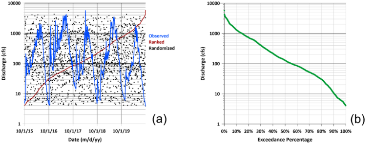
A single FDC, in fact, represents all permutations of the source dataset since the composition is the same regardless of the data time-based order. The permutation value is the number of ways to choose a sample of elements (r) from a set of distinct objects (n) when order matters and replacements are not allowed.
P(n,r) = n!/(n-r)! Eq (1)
where n = total number of objects, r = number of objects selected, and 0! = 1
Given a daily FDC with a one-year period for the source data, the number of possible arrangements is estimated to be P(365, 365) = 2.5 · 10778. For comparison, astrophysicists estimate the number of protons in the known universe, the Eddington number, as 1.5 · 1080 (Abramowicz, 2008). The challenge is clear – how is it possible to make an FDC unique to a specific dataset and to know if the source data meets the IID condition?
Enhanced Flow Duration Curve
There is a surprisingly simple solution that also provides additional information about the source dataset and addresses the IID issue. The answer is to use a lag(1) autocorrelation scatterplot in conjunction with an FDC and calculate the lag(1) autocorrelation coefficient, r(1).
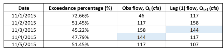
For this study, day-to-day pairings use a Qt, (flow for day “t”) and Qt+1 (flow for following day “t+1” ) system, where “1” represents one-day lag between the discharges. By using the Qt exceedance percentage for the x-axis and the Qt+1 discharge value for the y-axis, a unique overlay of next-day discharge points is possible for the FDC. Table 1 summarizes these values. Figure 2 shows the enhancement (compare to Figure 1b).
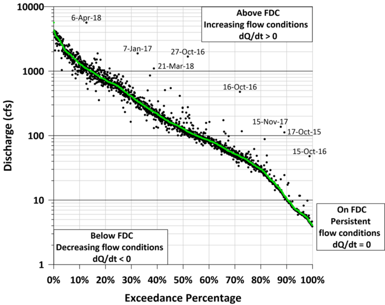
The spread of Qt+1 datapoints is key to visualizing the autocorrelation within the dataset. Points clustered along the FDC line indicate more persistent, stable conditions with higher autocorrelation, while increasingly scattered points indicate more random, flashier conditions with smaller autocorrelation.
This is consistent with Heckert and Filliben (2003) for describing a lag(1) autocorrelation scatterplot. They state that a tight clustering of data points along the (Qt = Qt+1) line is a signature of positive autocorrelation, indicating highly persistent conditions. Conversely, if the data points have a loose, dispersed pattern, it is a signature of lower autocorrelation and that the data are more random.
Conclusion
This short article is an introduction to the concept of an enhanced flow duration curve (EFDC) and some of its benefits. By combining two common hydrologic tools, the flow duration curve and the lag(1) autocorrelation scatterplot, a more informative graphic is now available.
Multiple applications include enhanced water resources management, improved detailed information about a river system, more targeted ecohydrology research projects, and new digital model evaluation methods, among other possibilities.
Remarks
The author thanks AIH for the opportunity to share this self-funded research.
Abramowicz, M. A., 1988, Eddington number and Eddington mass, The Observatory.
https://adsabs.harvard.edu/full/1988Obs…108…19A/0000019.000.html
Heckert, N., & Filliben, J., 2003. NIST/SEMATECH e-Handbook of Statistical Methods; Chapter 1: Exploratory Data Analysis.
https://doi.org/10.18434/M32189
Helsel, D.R., Hirsch, R. M., Ryberg, K. R., Archfield, S. A., & Gilroy, E. J. (2020).
Statistical Methods in Water Resources: U.S. Geological Survey Techniques and Methods, book 4.
https://doi.org/10.3133/tm4A3
Searcy, J.K., 1959. Flow-Duration Curves (Report No. 1542). US Government Printing Office.
https://pubs.usgs.gov/publication/wsp1542A